Thousands of (not-so) tiny SVDs: from 15 s to 66 ms on a GPU
In patch-denoise the main workload consist in computing a Singular Value Decomposition (SVD) of a lot of patches1 extracted from an fMRI volume, do some basic math on the singular values, to remove noise, and the recombine them. See more in [1].
Info
This is an approximate reconstitution on how the optimization went down. It was also my first try at doing code optimization with help of LLM (and later on, agents), more on this at the end.
Also, the true history of the optimization is a bit more complicated, and some gaps were LLM-filled to draft this post. There is an accompanying repository, to showcase the optimization steps.
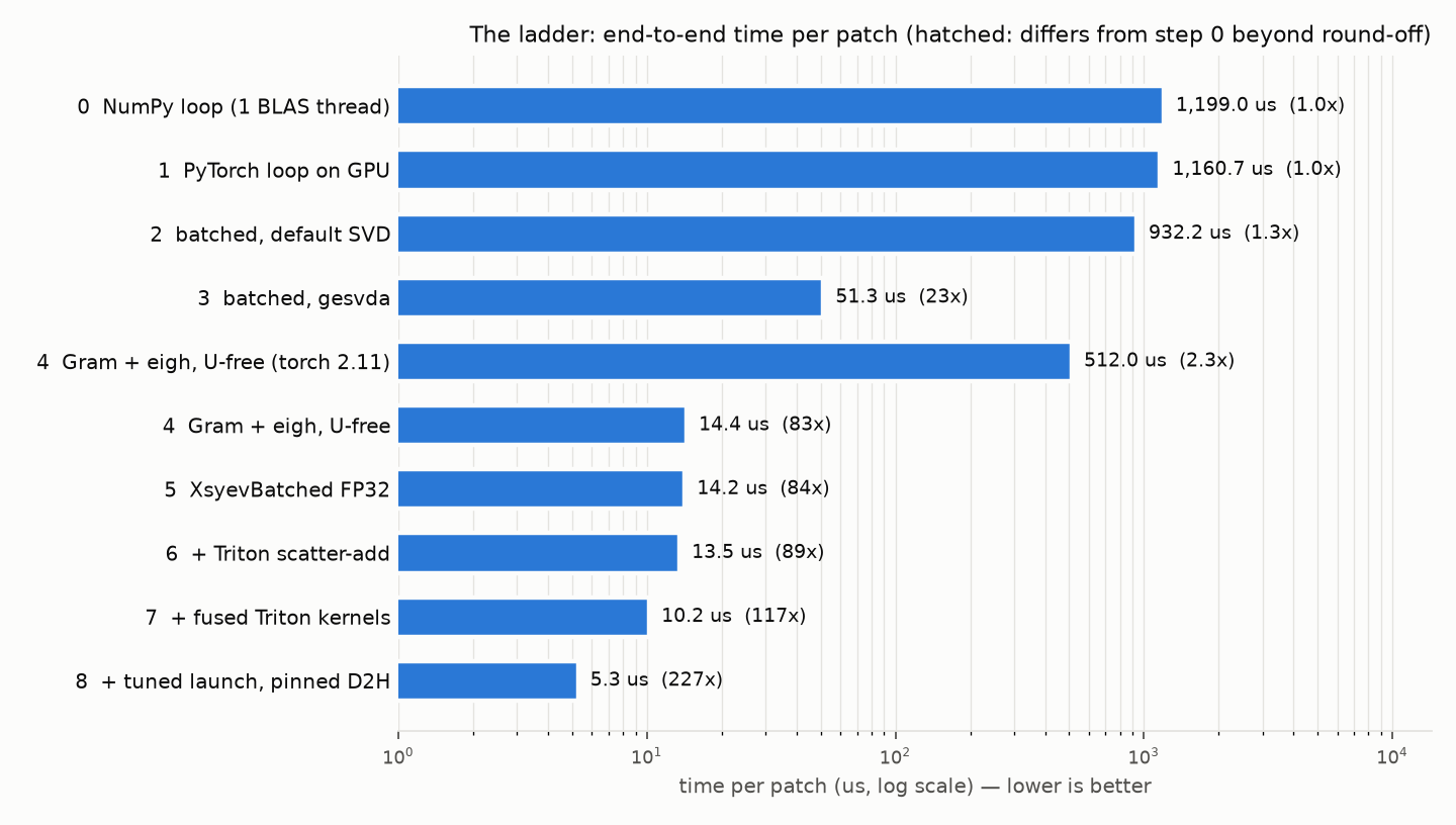
Figure 1: End-to-end time per patch for each step (log scale).
1. The workload
The motivating application is MP-PCA denoising of 4D MRI [2], but its details barely matter here. For this blog post just consider a convolution-style extraction of 3D+T patches. Each patch is unrolled in a Casorati matrix \(X \in \mathbb{R}^{N \times T}\), with \(N = 11^3 = 1331\) and \(T = 48\). For each patch:
- subtract each voxel's temporal mean: \(X_c = X - m \mathbf{1}^\top\);
- compute the singular values of \(X_c\) and choose a rank \(p\) from them,
- reconstruct \(\hat X = U_p S_p V_p^\top + m \mathbf{1}^\top\) and accumulate \(w \hat X\), with \(w = 1/(2+p)\), into the output volume.
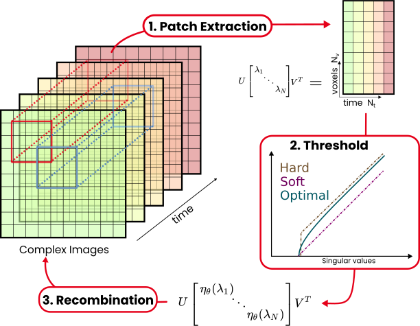
Figure 2: The denoising loop to optimize.
All numbers come from a companion repository with one self-contained script
per step (see Reproducing). Each step implements
denoise(np.ndarray) -> np.ndarray, is timed host to host (best of 5 after a
warm-up) and is checked against step 0's output. Timelines are Nsight Systems
traces rendered by tools/nsys_timeline.py. The setup:
- NVIDIA RTX 5000 Ada (32 GB), CUDA 13.0; AMD Threadripper PRO 7975WX, OpenBLAS 0.3.31
- PyTorch 2.14.1, Triton 3.8.0, nvmath-python 1.0.0
- a rank-5 phantom on a spatially varying baseline of about 1000, with Gaussian noise of standard deviation 4.
2. Step 0: the textbook loop
The naive implementation would look something like this:
def denoise(vol):
    out = np.zeros_like(vol)
    wsum = np.zeros(vol.shape[:3] + (1,), dtype=vol.dtype)
    for i, j, k in patch_corners():
        sl = np.s_[i : i + px, j : j + py, k : k + pz]
        x = vol[sl].reshape(-1, vol.shape[-1])  # (N, T)
        m = x.mean(axis=1, keepdims=True)
        u, s, vt = np.linalg.svd(x - m, full_matrices=False)
        p = mp_rank(s[:-1], x.shape[0])  # s[-1] == 0: the null direction
        xd = (u[:, :p] * s[:p]) @ vt[:p] + m
        w = 1.0 / (2.0 + p)
        out[sl] += w * xd.reshape(px, py, pz, -1)
        wsum[sl] += w
    return out / np.maximum(wsum, 1e-12)
One CPU detail first: OpenBLAS's default threading hurts on matrices this
small. One 1331 x 48 SVD takes 1.7 ms on 1 thread, 2.2 ms on 4 and 6.3 ms on
64 (micro/cpu_threads.py). The fair baseline is therefore single-threaded:
15.1 s, 1.2 ms per patch. One process per core would give roughly 30x; we
take the GPU route instead.
3. Step 1: the naive GPU port
Replace np with torch and upload the volume once. Result: 14.6 s, 3%
faster, on a GPU that can do 65 TFLOPS.
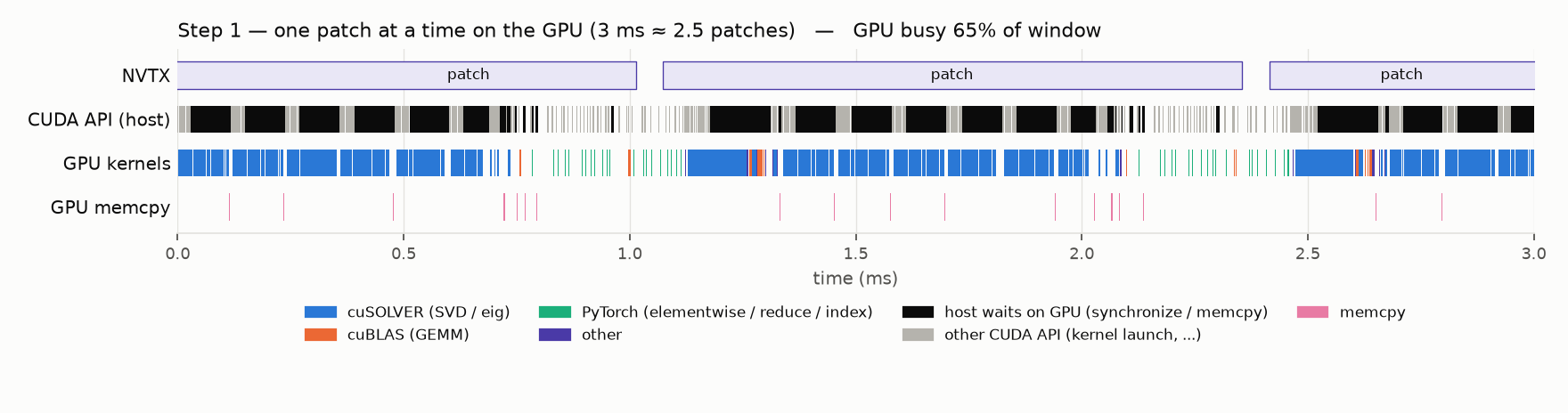
Figure 3: Step 1, about 2.5 patches. Each patch takes about 150 kernel launches and 12 blocking device-to-host copies.
On CUDA, torch.linalg.svd defaults to cuSOLVER's Jacobi solver
(gesvdj). For one 1331 x 48 matrix it issues about 150 microsecond-sized
kernels, and between sweeps it copies a convergence flag back to the host and
waits for it (the black bars). Reading \(p\) back for the slicing adds one more
sync per patch. The GPU solves one tiny problem at a time and is mostly idle.
4. Step 2: batching
Sending patch one by one to the GPU is driving a lot of back and forth between the host (CPU) and device (GPU), and we keep going back into Python userland, closing slowdown, could we minimize this and launch as much compute as possible at once ?
The answer to this batching: send a Batch of patch of size (B,N,T) at once, and process it together:
def mppca_batch(x):
    """MP-PCA on a (B, N, T) batch. Returns (denoised, rank)."""
    _, n, t = x.shape
    m = x.mean(dim=2, keepdim=True)  # temporal mean of each voxel
    u, s, vh = torch.linalg.svd(x - m, full_matrices=False, driver=SVD_DRIVER)
    t -= 1  # drop the null direction (constant time course)
    u, s, vh = u[..., :t], s[:, :t], vh[:, :t]

    eigs = s**2 / n
    rcum = eigs.flip(-1).cumsum(-1).flip(-1)
    p_range = torch.arange(t, device=x.device)
    signal = (eigs - eigs[:, -1:]) * (t - p_range) * (n - p_range) > 4 * rcum * (
        t * n
    ) ** 0.5
    p = signal.sum(-1)
    s_kept = s * (p_range < p[:, None])
    return torch.baddbmm(m, u * s_kept[:, None, :], vh), p

def patch_row_indices(vol_shape, device):
    _, ny, nz, _ = vol_shape
    corners = torch.from_numpy(patch_corners()).to(device)
    base = (corners * torch.tensor([ny * nz, nz, 1], device=device)).sum(-1)
    ox, oy, oz = torch.meshgrid(*(torch.arange(p, device=device) for p in PATCH), indexing="ij")
    offsets = (ox * ny * nz + oy * nz + oz).reshape(-1)
    return base[:, None] + offsets  # (P, N)


def denoise(vol):
    vol = torch.from_numpy(vol_np).cuda()
    t = vol.shape[-1]
    flat = vol.view(-1, t)
    out = torch.zeros_like(flat)
    wsum = torch.zeros(flat.shape[0], device="cuda")
    rows = patch_row_indices(vol.shape, "cuda")
    for b in range(0, rows.shape[0], BATCH):
        idx = rows[b : b + BATCH]
        x = flat[idx]  # (B, N, T)
        xd, p = mppca_batch(x)
        w = 1.0 / (2.0 + p.float())
        out.index_add_(0, idx.reshape(-1), (xd * w[:, None, None]).reshape(-1, t))
        wsum.index_add_(0, idx.reshape(-1), w.repeat_interleave(idx.shape[1]))
    return (out / wsum.clamp_min(1e-12)[:, None]).view(vol.shape).cpu().numpy()
Using batching: 11.7 s overall. The batched default is still Jacobi, still checking convergence on the host between sweeps, and Jacobi is designed for small square matrices, not 1331 x 48 ones.
torch.linalg.svd takes a driver argument, so measure them all:
torch.linalg.svd driver |
us/patch |
|---|---|
| default | 865.17 |
gesvd |
1441.06 |
gesvdj |
864.89 |
gesvda |
41.06 |
5. Step 3: driver = "gesvda"
gesvda is cuSOLVER's approximate SVD for batches of tall-skinny matrices: it
forms the Gram matrix, eigendecomposes it and recovers U, which is the right
algorithm for \(N \gg T\). Switching this single argument brings us down to 646 ms, 23x over step
0.
It would be totally fine to stop here in term of optimization (and for a while this is what I did), but what if it could go faster ? At on point I ran the profiler on the base code and found out that in gesvda most of the computations happens in float64, and this is a big no-no in GPU optimization. 2
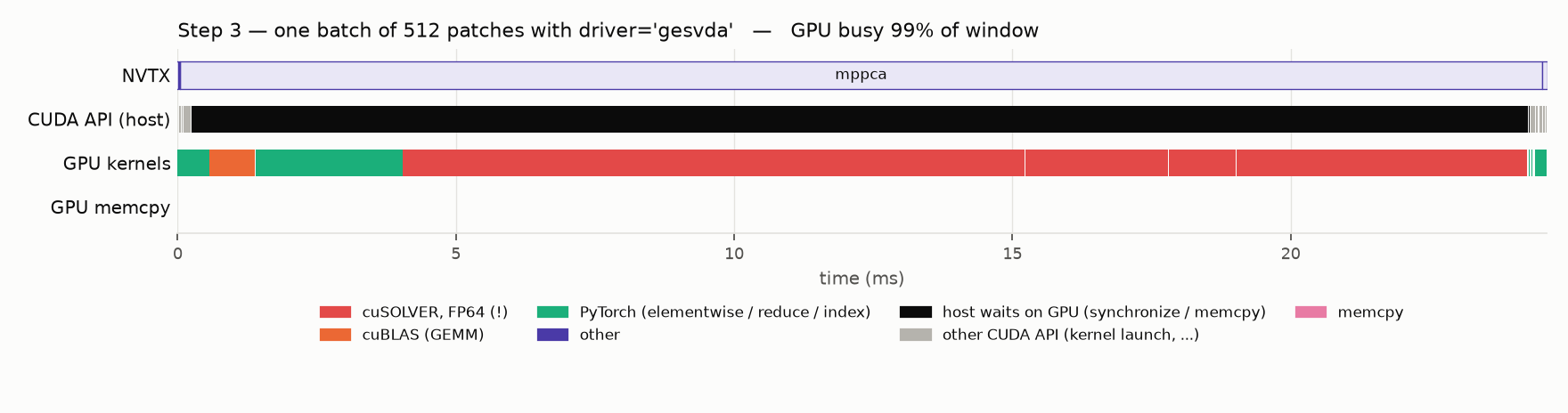
Figure 4: Step 3, one batch of 512 patches. Red means kernels templated on double, on float32 input.
The kernel names give it away: cutlass_80_tensorop_d884gemm,
laed4_par<...double...>, sytrd4_cta<sytrd_params<double,...>>. On float32
input, cusolverDnSgesvdaStridedBatched computes the Gram matrix, the
eigendecomposition and the back-transform in FP64, as NVIDIA documents it
(B = A^T A by DGEMM, eig(B) in double).
| GPU time (ms) | step 3 |
|---|---|
| cuSOLVER, FP64 | 497.4 |
| cuBLAS (GEMM) | 20.0 |
| PyTorch (elementwise / reduce / index) | 84.3 |
| memcpy D2H | 32.7 |
| total | 638.1 |
Note
Why is NVIDIA forcing us in FP64 ?
I have no definitive answer, but my main assumption is for numerical precision and stability, The gram matrix \(A^T A\) of tall and skinny matrices can badly conditioned (its condition number is the square of the one of \(A\)) notably if they have a large DC offset.
Luckily enough, we are already removing the DC offset, and so maybe we can just do the SVD manually ?
6. Step 4: do gesvda's job in FP32, and skip U
For \(N \gg T\), everything needed is in the \(T \times T\) Gram matrix:
\[ G = X_c^\top X_c = V \,\mathrm{diag}(s^2)\, V^\top . \]
Its eigenvalues are the squared singular values, and \(\mathbf{1}/\sqrt{T}\) is the null eigenvector, always first in ascending order. U is not needed either, because the reconstruction only projects the rows of \(X_c\):
\[ U_p S_p V_p^\top = X_c V_p V_p^\top = X_c P, \qquad P = V_p V_p^\top \in \mathbb{R}^{T\times T}. \]
A patch now costs a Gram GEMM, a small \(T \times T\) eigendecomposition and one
reconstruction GEMM, with the + m fused in through baddbmm:
def mppca_batch(x):
    _, n, _ = x.shape
    m = x.mean(dim=2, keepdim=True)          # temporal mean of each voxel
    xc = x - m
    lam, v = torch.linalg.eigh(xc.mT @ xc)  # ascending, V in columns
    keep, p = mp_keep(lam, n)               # 0/1 mask; lam[:, 0] (null) never kept
    proj = (v * keep[:, None, :]) @ v.mT    # V_p V_p^T
    return torch.baddbmm(m, xc, proj), p
Unfortunately, the performance here depends on the pytorch version:
- PyTorch 2.11 dispatches batched
eighto Jacobi (syevjBatched, thousands of launches per batch): and we are slow again, 6.5 s, ten times slower thangesvda; - PyTorch 2.14 dispatches to cuSOLVER's batched divide and conquer
(
sytrd4_cta<float>,laed4_par,steqr_ker), in FP32: 182 ms, 83x.
7. Step 5: calling cusolverDnXsyevBatched directly
Before PyTorch 2.14, you have to call the fast routine yourself.
cusolverDnXsyevBatched (CUDA 12.6+) is cuSOLVER's 64-bit generic API with an
explicit compute type. PyTorch does not expose it, but nvmath-python ships
Cython bindings generated from the cuSOLVER headers.
import torch
import nvmath.bindings.cublas as cublas
import nvmath.bindings.cusolver as cusolver
import nvmath.bindings.cusolverDn as cusolverDn

class XsyevBatched:
    def __init__(self, batch, t, device="cuda"):
        self.batch, self.t = batch, t
        self.handle = cusolverDn.create()
        self.params = cusolverDn.create_params()
        g = torch.empty(batch, t, t, device=device)
        self.w = torch.empty(batch, t, device=device)
        self.info = torch.empty(batch, dtype=torch.int32, device=device)
        args = (cusolver.EigMode.VECTOR, cublas.FillMode.LOWER, t, CUDA_R_32F)
        dev_bytes, host_bytes = cusolverDn.xsyev_batched_buffer_size(
            self.handle, self.params, *args, g.data_ptr(), t,
            CUDA_R_32F, self.w.data_ptr(), CUDA_R_32F, batch)
        self.dev_ws = torch.empty(max(dev_bytes, 1), dtype=torch.uint8, device=device)
        self.host_ws = torch.empty(max(host_bytes, 1), dtype=torch.uint8)
        self._args = args

    def __call__(self, g):
        cusolverDn.set_stream(self.handle, torch.cuda.current_stream().cuda_stream)
        cusolverDn.xsyev_batched(self.handle, self.params, *self._args,
            g.data_ptr(), self.t, CUDA_R_32F, self.w.data_ptr(), CUDA_R_32F,
            self.dev_ws.data_ptr(), self.dev_ws.numel(),
            self.host_ws.data_ptr(), self.host_ws.numel(),
            self.info.data_ptr(), self.batch)
        return self.w  # g now holds the eigenvectors
Two pitfalls:
- We have to create a dedicated object to hold the configuration "workspace" of the Eigendecompsoition (which depends on the batch and size of the Gram matrix).
- cuSOLVER is column-major by default, so we need to transpose back the results, the eigenvectors comes back as rows.
We get similar speed as in step 4: 179 ms. There is an extra advantage of using this custom setup, event for Pytorch 2.14 and above:
The info tensor is never read back on CPU (it holds convergences checks), we blindly trust the process and don't need to read it (Pytorch implementation does, causing a host synchronization). Here nothing synchronize, and the GPU queues up work as much as possible !
8. Step 6: a Triton scatter-add
With SVD decomposition optimized to the max , our attention moves to the recombination step: With the different baddmm and index_add_ steps, this creates a lot of back and forth between shared memory and cache layers, we also keep an int64 index tensor that could be computed on the fly from the patch corner. The solution is to deploy a Triton kernel to do both indexadd jointly, and
import triton
import torch
import triton.language as tl

@triton.jit
def _patch_rows(base, n, ny, nz, PY: tl.constexpr, PZ: tl.constexpr):
    """Voxel ``n`` of a patch whose first voxel is ``base`` -> volume row."""
    return base + (n // (PY * PZ)) * ny * nz + (n // PZ % PY) * nz + n % PZ

@triton.jit
def scatter_add_kernel(
    out_ptr, wsum_ptr, xd_ptr, w_ptr, base_ptr,
    ny, nz, T,
    PX: tl.constexpr, PY: tl.constexpr, PZ: tl.constexpr,
    BLOCK_N: tl.constexpr, BLOCK_T: tl.constexpr,
):  # fmt: skip
    """out[rows] += w * xd[b], wsum[rows] += w, for patch b and a block of rows."""
    b = tl.program_id(0)
    n = tl.program_id(1) * BLOCK_N + tl.arange(0, BLOCK_N)
    t = tl.arange(0, BLOCK_T)
    n_mask = n < PX * PY * PZ
    mask = n_mask[:, None] & (t < T)[None, :]

    # voxel n of the patch -> row of the (X*Y*Z, T) volume
    row = _patch_rows(base, n, ny, nz, PY, PZ)
    w = tl.load(w_ptr + b)

    xd = tl.load(xd_ptr + (b * PX * PY * PZ + n[:, None]) * T + t[None, :], mask=mask)
    tl.atomic_add(out_ptr + row[:, None] * T + t[None, :], w * xd, mask=mask)
    tl.atomic_add(wsum_ptr + row, w + tl.zeros_like(row).to(tl.float32), mask=n_mask)

def scatter_add(out, wsum, xd, w, base, vol_shape):
    b, n, t = xd.shape
    _, ny, nz, _ = vol_shape
    block_n = 64
    scatter_add_kernel[(b, triton.cdiv(n, block_n))](
        out, wsum, xd, w, base, ny, nz, t, *PATCH,
        BLOCK_N=block_n, BLOCK_T=triton.next_power_of_2(t),
    )
This only help a little (Runtime: 170 ms, a 5% improvement), but it brings up the next idea: A kernel that compute patch adresses can also read the patch straight from the volume, and we don't need to materialize the batch !
9. Step 7: never materialize the batch
Two kernels read patches directly from the volume. Between them, only \(T \times T\)-sized tensors exist.
Kernel 1 computes the centered Gram matrix, one program per patch. A tile
spans whole rows (BLOCK_T ≥ T), so each voxel's temporal mean is a row
reduction in registers and the kernel makes a single pass over the patch.
Centering over voxels would need a first pass just for the mean.
@triton.jit
def gram_kernel(vol_ptr, base_ptr, gram_ptr, ny, nz, T,
                PX: tl.constexpr, PY: tl.constexpr, PZ: tl.constexpr,
                BLOCK_N: tl.constexpr, BLOCK_T: tl.constexpr):
    b = tl.program_id(0)
    base = tl.load(base_ptr + b)
    t = tl.arange(0, BLOCK_T)
    t_mask = t < T
    N: tl.constexpr = PX * PY * PZ

    gram = tl.zeros((BLOCK_T, BLOCK_T), dtype=tl.float32)
    for n0 in range(0, N, BLOCK_N):
        n = n0 + tl.arange(0, BLOCK_N)
        mask = (n < N)[:, None] & t_mask[None, :]
        row = _patch_rows(base, n, ny, nz, PY, PZ)
        x = tl.load(vol_ptr + row[:, None] * T + t[None, :], mask=mask, other=0.0)
        m = tl.sum(x, 1) / T  # temporal mean of each voxel: a row reduction
        xc = tl.where(mask, x - m[:, None], 0.0)
        gram = tl.dot(tl.trans(xc), xc, gram, input_precision="ieee")
    g_ptrs = gram_ptr + b * T * T + t[:, None] * T + t[None, :]
    tl.store(g_ptrs, gram, mask=t_mask[:, None] & t_mask[None, :])
Kernel 2, one program per patch and block of voxels, recomputes \(m\) the same way, forms \(w\,(X_c P + m)\), and adds it and \(w\) atomically into the output and weight volumes:
x = tl.load(vol_ptr + row[:, None] * T + t[None, :], mask=mask, other=0.0)
m = tl.sum(x, 1) / T
xc = tl.where(mask, x - m[:, None], 0.0)
xd = tl.dot(xc, proj, input_precision="ieee") + m[:, None]
tl.atomic_add(out_ptr + row[:, None] * T + t[None, :], w * xd, mask=mask)
tl.atomic_add(wsum_ptr + row, w + tl.zeros_like(row).to(tl.float32), mask=n_mask)
input_precision="ieee" is deliberate: using TF32 would speed up both dots, but
throw away the precision we wanted to keep in Step 4 where we started to decompose the SVD computations.
Result: 129 ms, 117x. GPU time falls from 173 to 118 ms, of which 39 ms is our two kernels. The 33 ms device-to-host copy is now more than a quarter.
10. Step 8: read the timeline, then tune
Launch configuration. Kernel 2 ran with Triton's defaults. A sweep over tile size and warps:
BLOCK_N |
2 warps | 4 warps | 8 warps |
|---|---|---|---|
| 32 | 1521 | 832 | 566 |
| 64 | 1781 | 1469 (step 7) | 1011 |
| 128 | 3142 | 1719 | 1063 |
Smaller tiles put more programs in flight to hide the latency of the atomics:
2.6x on this kernel, and 10% on the Gram kernel with BLOCK_N=32. Contention
between overlapping patches, on the other hand, is not the problem:
reordering patches so that no two in a batch overlap made the call slower (144
vs. 126 ms), because neighbouring patches share lines in L2.
Pinned output. .cpu() copies 85 MB into pageable memory, which the driver
stages through a bounce buffer: 36.6 ms. Copying into pinned memory takes 3.1
ms, and allocating the pinned buffer on every call is free after the first one,
because PyTorch's caching host allocator reuses it:
host = torch.empty(out.shape, pin_memory=True)  # cached by torch's host allocator
host.copy_(out / wsum.clamp_min(1e-12)[..., None])
return host.numpy()
Batch size. The fused pipeline has fixed costs per batch: about ten
launches, plus torch.linalg.eigh blocking the host while it reads back
info. Only \((B, T, T)\) tensors live per batch, so large batches cost almost
no memory: 147 ms at 64 patches per batch, 75 ms at 512, 67 ms at 2048.
Step 8 uses 2048.
Result: 66.5 ms, 227x over step 0, 5.3 µs per patch, matching step 0 to 1.6e-7.
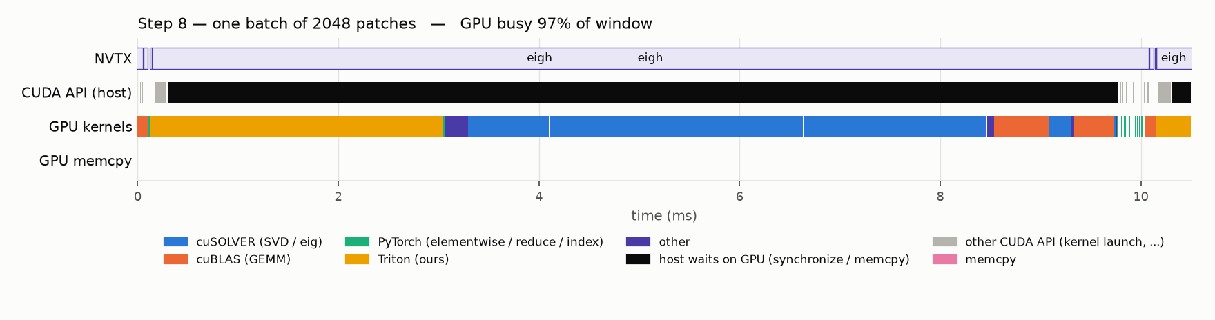
Figure 5: Step 8, one batch of 2048 patches: our Gram kernel, the eigensolver (blue, now the largest item), then the projector GEMMs and the reconstruction kernel of the next batch.
| GPU time (ms) | step 5 | step 7 | step 8 |
|---|---|---|---|
| cuSOLVER (eig) | 33.1 | 33.0 | 33.5 |
| cuBLAS (GEMM) | 41.9 | 6.3 | 6.5 |
| PyTorch | 58.7 | 1.8 | 1.0 |
| Triton (ours) | 0.0 | 39.3 | 18.1 |
| memcpy H2D | 3.5 | 3.5 | 3.5 |
| memcpy D2H | 33.4 | 32.5 | 3.1 |
| total | 172.8 | 118.4 | 67.8 |
The eigensolver is now half of the GPU time🎉. And we likely hit the bottom here, so time to wrap it up.
11. Summary
| step | time (ms) | us/patch | vs. step 0 | rel. err. vs. step 0 |
|---|---|---|---|---|
| 0 NumPy loop (1 BLAS thread) | 15,107.2 | 1,198.98 | 1.0x | 0.0e+00 |
| 1 PyTorch loop on GPU | 14,624.9 | 1,160.71 | 1.0x | 6.5e-07 |
| 2 batched, default SVD | 11,746.1 | 932.23 | 1.3x | 6.5e-07 |
3 batched, gesvda |
645.8 | 51.25 | 23x | 1.1e-07 |
| 4 Gram + eigh, U-free (torch 2.11) | 6,450.9 | 511.98 | 2.3x | 1.4e-07 |
| 4 Gram + eigh, U-free (torch 2.14) | 181.8 | 14.43 | 83x | 1.1e-07 |
5 XsyevBatched FP32 |
178.8 | 14.19 | 84x | 1.1e-07 |
| 6 + Triton scatter-add | 170.3 | 13.52 | 89x | 1.4e-07 |
| 7 + fused Triton kernels | 128.6 | 10.21 | 117x | 1.5e-07 |
| 8 + tuned launch, pinned D2H | 66.5 | 5.28 | 227x | 1.6e-07 |
- Batched does not mean fast. The routine behind the batch decides everything, iJacobi vs. divide and conquer was a 20 → 100x improvement, and was dependent on a Pytorch version as well.
- Profile before believing a speedup.
gesvdawas a 23x win and still spent 78% of its time in FP64. - Don't compute what you don't need. For \(N \gg T\), eigendecompose the \(T \times T\) Gram matrix (the svda approach) and save computations as much as possible.
Note
About Agentic optimization
The story this blog post tells is also a story on me tipping a toe in "agentic engineering". In this context it felt easy, notably because I already had tests in place to check numerical accuracy, and the prompts were mostly, "make <this> faster, I think you should use <that>", as well as running the nsight system profiler. This mostly appended in August 2026 when I had spare time, and using Sonnet 5. Maybe using something like autoresearch, b would provide similar results, maybe even faster.
Overall I felt this mostly as an acceleration and improvement on the quality I was able to reach (I got further and faster that I would I have hoped for), and also was the opportunity to get familliar with Triton (I am probably never going to write a C++ CUDA Kernel by hand anymore, but having to do so in my undergrad study is surely why it felt so easy to move to triton). Yet, I haven't been felt "replaced" by Claude Code or Codex, I wonder if this feeling will last.
12. Reproducing
See the accompanying repository. If you want to just denoise stuff super fast, check paquiteau/patch-denoising
uv sync
./run_all.sh                         # every step, results/summary.org, ladder.png
uv run python micro/svd_drivers.py   # and likewise for the other micro/ scripts
tools/profile.sh step8_tuned         # nsys capture of one warm call -> results/prof/